This is a follow-on from a previous post on tangent spaces. It is part of a series of posts that I write on the basics of differential or Riemannian geometry, providing the necessary background for reading some of the more advanced textbooks on general relativity. I will introduce the derivative of a smooth map between manifolds and work a little bit with the definition(s) to become familiar with the thicket of mathematical notation. Then I narrow in on the special case where \(f\) is a real-valued function, introduce the notions of dual space and covectors, and finally show the connection to the differential known from basic calculus.
Defining the Derivative
Having established tangent spaces and smooth maps between manifolds, we are now in a position to define the derivative of a smooth map \(f\) between manifolds. In some sense, this is where analysis on manifolds begins. The map \(f\) induces a linear transformation between the tangent spaces of the manifolds and is therefore also called tangent map. We offer two independent definitions and show that they give the same result.
Definition: Derivative (Differential, Tangent Map, Jacobian)
Let \(\mathcal{M}\) and \(\mathcal{N}\) be two differentiable manifolds, and let \(f : \mathcal{M} \to \mathcal{N}\) be a smooth map.
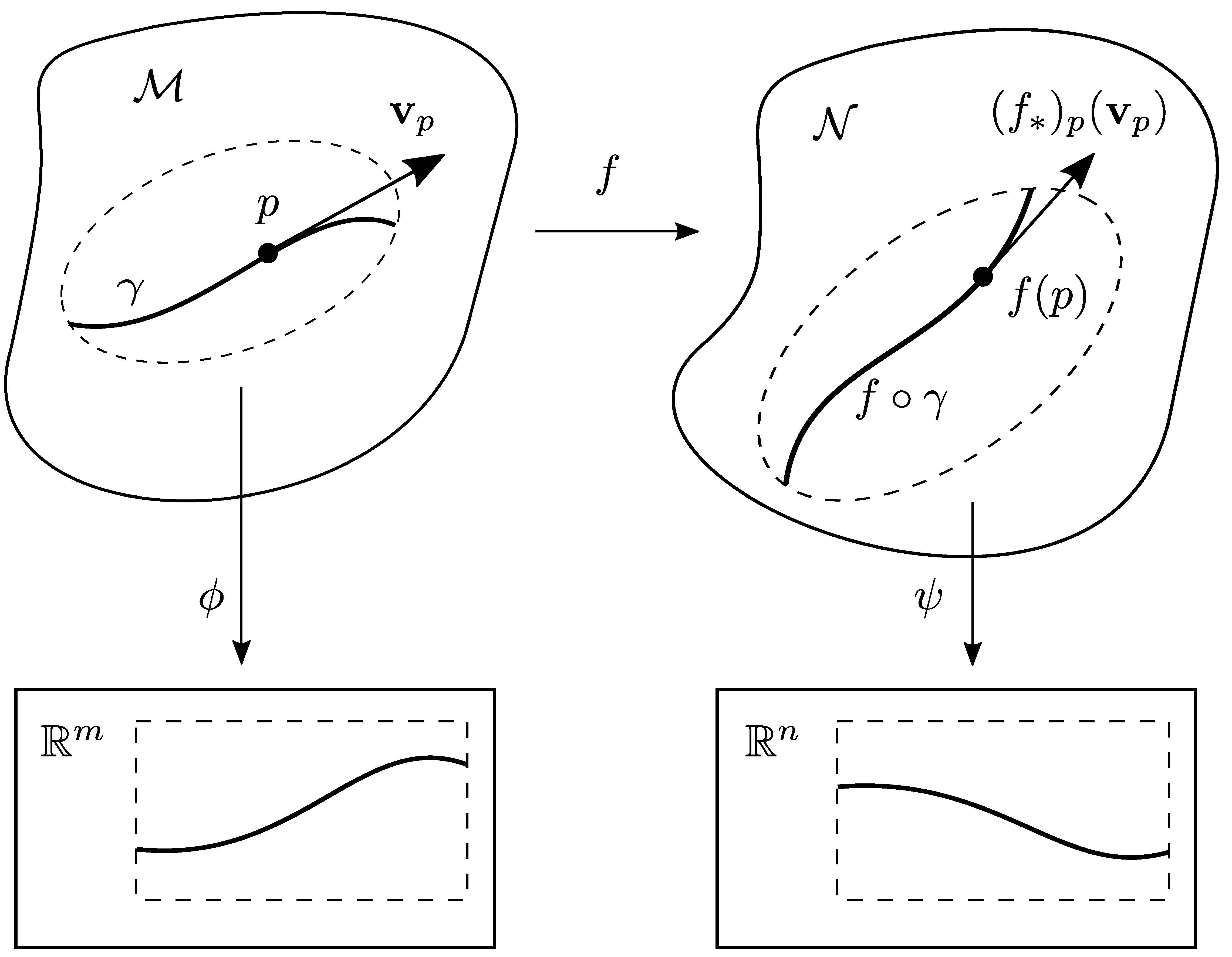
At each \(p \in \mathcal{M}\) the map \(f\) induces a linear transformation between the tangent spaces,
\[ \begin{aligned} (f_*)_p : T_p \mathcal{M} &\to T_{f(p)} \mathcal{N} \ , \\[0.3em] \textrm{D}_\gamma &\mapsto \textrm{D}_{f\circ\gamma} \ , \end{aligned} \]
which is called the derivative of \(f\) at \(p\) and intended to serve as ''linear approximation to \(f\) near \(p\).'' The derivative is also called differential, tangent map, or Jacobian and alternatively denoted by \((f_*)_p\), \((df)_p\), \(Df\), or \(f'\). The term 'differential' and the notation \((df)_p\) are often reserved for the case \(\mathcal{N}=\mathbb{R}\).
The following definitions are equivalent:
- For \(\mathbf{v}_p \in T_p \mathcal{M}\), we define \((f_*)_p\) to be the derivation on \(\mathcal{F}_{f(p)} \mathcal{N}\) which is for all \(g \in \mathcal{F}_{f(p)} \mathcal{N}\) defined by
\[\big((f_*)_p(\mathbf{v}_p)\big)(g) = \mathbf{v}_p(g \circ f) \ .\]
For \(\mathbf{v}_p \in T_p \mathcal{M}\) we select a smooth curve \(\gamma\) in \(\mathcal{M}\) with \(\gamma(0) = p\) and \(d_\tau \gamma|_{\tau=0} = \dot{\gamma}(0) = \mathbf{v}_p\). Then \(f\circ\gamma\) is a smooth curve in \(\mathcal{N}\) through \(f(p)\) at \(t=0\) and we define
\[(f_*)_p(\mathbf{v}_p) = \frac{d}{d\tau} (f \circ \gamma) \Big|_{\tau=0} = (f \circ \gamma)'(0) \ .\]
Sometimes \(f_*(\mathbf{v})\) is also called the (pointwise) pushforward of \(\mathbf{v}\) by \(f\) because it ``pushes'' tangent vectors forward from the domain manifold to the codomain. You can also define a (global) pushforward between tangent bundles of the corresponding manifolds.
The following Figure may help untangle the notation. Observe that in the first definition, \((f_*)_p\) is well-defined and obviously a linear transformation, but not obviously a tangent vector at \(f(p)\), whereas, in the second definition, \((f_*)_p\) is clearly a tangent vector, but not obviously independent of the choice of \(\gamma\).
Let's play a little bit with these definitions!
How can one prove directly, using the first definition, that \((f_*)_p(\mathbf{v}_p)\) is a derivation (or tangent vector) at \(f(p)\), i.e., \((f_*)_p(\mathbf{v}_p) \in T_{f(p)}(\mathcal{N})\)? We need to show for \((f_*)_p(\mathbf{v}_p)\) that the linearity properties and the product rule hold. Let's illustrate the product rule. The key step happens in the third line where we rely on the fact that \(\mathbf{v}_p\) is a derivation at \(p\) and the product rule for \(\mathbf{v}_p\) thus holds:
\[ \begin{aligned} \big((f_*)_p(\mathbf{v}_p)\big)[g_1 \cdot g_2] &= \mathbf{v}_p [(g_1 \cdot g_2) \circ f] \\[0.5em] &= \mathbf{v}_p [(g_1 \circ f) \cdot (g_2 \circ f)] \\[0.5em] &= (g_1 \circ f)(p) \;\mathbf{v}_p [g_2 \circ f] + (g_2 \circ f)(p) \;\mathbf{v}_p [g_1 \circ f] \\[0.5em] &= g_1(f(p)) \big((f_*)_p(\mathbf{v}_p)\big)[g_2] + g_2(f(p)) \big((f_*)_p(\mathbf{v}_p)\big)[g_1] \ . \end{aligned} \]
We can also show easily that \((f_*)_p(\mathbf{v}_p)\) is linear:
\[ \begin{aligned} (f_*)_p(a\mathbf{v}_p + b\mathbf{w}_p)(g) &= a\mathbf{v}_p(g \circ f) + b\mathbf{w}_p(g \circ f) \\[0.5em] &= a (f_*)_p (\mathbf{v}_p)(g) + b (f_*)_p (\mathbf{w}_p)(g) \ . \end{aligned} \]
How does one get from definition #2 to definition #1? We need to show that, at each \(p \in \mathcal{M}\), the function \(f_*\) satisfies \((f_*)_p(\mathbf{v}_p)(g) = \mathbf{v}_p (g\circ f)\) for every vector \(\mathbf{v}_p \in T_p\mathcal{M}\) and every function \(g\) from \(\mathcal{N}\) into \(\mathbb{R}\), defined in a neighborhood of \(f(p)\). We have
\[ \begin{aligned} (f_*)_p(\mathbf{v}_p)(g) &= (f_*)_p (\textrm{D}_{\gamma})(g) = \textrm{D}_{f\circ\gamma}(g) \\[0.5em] &= \frac{d}{d\tau} (g \circ f \circ \gamma)(\tau) \Big|_{\tau=0} \\[0.5em] &= \textrm{D}_{\gamma}(g \circ f) = \mathbf{v}_p (g\circ f) \ . \end{aligned} \]
Everything done so far was independent of any coordinate system near \(p\) or \(f(p)\). For the following considerations, however, we introduce charts \((U,\phi)\) around \(p\) on \(\mathcal{M}\) with coordinates \(\left\lbrace x^i \right\rbrace_{i=1}^m\) and \((V,\psi)\) around \(f(p)\) on \(\mathcal{N}\) with coordinates \(\left\lbrace y^j \right\rbrace_{j=1}^n\), in order to show two things:
- The definition \((f_*)_p(\mathbf{v}_p) = (f \circ \gamma)'(0)\) does not depend on the choice of the curve \(\gamma\).
- By working in coordinate charts we can define a matrix that represents \((f_*)_p\), called the Jacobian.
Again, the above Figure may help to stay oriented in the thicket of mathematical notation. The curve \(\gamma\) is given by
\[ \gamma(\tau) = (\phi\circ\gamma)(\tau) = \big(x^1(\tau), \dots , x^m(\tau)\big) \ , \]
and the curve
\[ f\circ\gamma : (-\epsilon,\epsilon) \to \mathcal{N} \]
is given by
\[ \begin{aligned} (f\circ\gamma)(\tau) &= \big(\psi\circ f\circ \phi^{-1}\big)\big(x^1(\tau), \dots , x^m(\tau) \big) \\[0.5em] &= \big( y^1(x(\tau)), \dots , y^n(x(\tau)) \big) \\[0.5em] &\overset{\text{s.c.}}{=} y^j\big(x(\tau)\big) \, \frac{\partial}{\partial y^j}\Big|_{f(p)} \ , \end{aligned} \]
where, in the last step, we have used the summation convention to write the vector as a sum of components multiplying differential operators that serve as basis vectors. Then \((f\circ\gamma)'(0)\) is the tangent vector in \(T_{f(p)}\mathcal{N}\) given by
\[ \begin{aligned} (f\circ\gamma)'(0) &= \frac{d}{d\tau} (f \circ \gamma) \Big|_{\tau=0} \\[0.5em] &= \Bigg( \frac{d x^i}{d\tau}\Big|_{\tau=0} \frac{\partial y^j}{\partial x^i}\Big|_{x(0)} \Bigg) \frac{\partial}{\partial y^j}\Big|_{f(p)} \\[0.5em] &= \Bigg( v^i \ \frac{\partial y^j}{\partial x^i}\Big|_{x(0)} \Bigg) \frac{\partial}{\partial y^j}\Big|_{f(p)} \\[0.5em] &= \, w^j \, \frac{\partial}{\partial y^j}\Big|_{f(p)} \ , \end{aligned} \]
where the \(v^i\) are the components of \(\mathbf{v}_p\) in the basis associated to \((U,\phi)\). Hence, \(\mathbf{w}_{f(p)} = (f_*)_p(\mathbf{v}_p) = (f\circ\gamma)'(0)\) does not depend on the choice of \(\gamma\), as long as \(\gamma'(0) = \mathbf{v}_p\).
The components of \(\mathbf{w}_{f(p)} = (f_*)_p(\mathbf{v}_p)\) in the basis associated to \((V,\psi)\) are
\[ w^j = \Bigg[ \frac{\partial y^j}{\partial x^i} \Bigg] v^i \ , \]
where \([\partial y^j / \partial x^i]\) is an \(m\times n\) matrix, the Jacobian matrix of the local representation of \(f\) at \(\phi(p)\).
Differential and Dual Space
Let's look at the special case \(\mathcal{N}=\mathbb{R}\) where we are dealing with a real-valued function \(f \in \mathcal{F}_p \mathcal{M}\), or \(f : \mathcal{M} \to \mathbb{R}\). Then \((f_*)_p : T_p\mathcal{M} \to T_{f(p)}\mathbb{R}\). But \(T_{f(p)}\mathbb{R}\) is spanned by the single coordinate vector \(\frac{d}{d y}\big|_{f(p)}\), so every \((f_*)_p(\mathbf{v}_p) \in T_{f(p)}\mathbb{R}\) is a multiple of \(\frac{d}{d y}\big|_{f(p)}\),
\[ (f_*)_p(\mathbf{v}_p) = w \,\frac{d}{d y}\Big|_{f(p)} \ . \]
We choose an arbitrary function \(g:\mathbb{R}\to\mathbb{R}\) to determine the coefficient \(w\):
\[ (f_*)_p(\mathbf{v}_p)(g) = \mathbf{v}_p(g \circ f) = w \,\frac{dg}{d y}\Big|_{f(p)} \ . \]
Specfically, we may choose \(g(y)=y\), i.e., the identify function, with \(dg/dy=1\):
\[ \begin{aligned} (f_*)_p(\mathbf{v}_p)(g) &= \mathbf{v}_p(g \circ f) \: = w \,\frac{dg}{d y}\Big|_{f(p)} \\[0.3em] &= \mathbf{v}_p(\mathrm{id} \circ f) = w \cdot 1 \\[0.8em] &= \mathbf{v}_p(f) = w \ . \end{aligned} \]
Thus, \(\mathbf{v}(f)\) completely determines \((f_*)(\mathbf{v})\) for all \(\mathbf{v} \in T_p\mathcal{M}\):
\[ (f_*)_p(\mathbf{v}) = \mathbf{v}(f) \,\frac{d}{d y}\Big|_{f(p)} \ . \]
Since \(T_{f(p)}\mathbb{R}\) is a flat one-dimensional vector space, all vectors are the same up to scaling and there is no need to write \((d/dy)|_{f(p)}\). Now, for this case \(f : \mathcal{M} \to \mathbb{R}\), we preferably use the term differential of \(f\) at \(p\), which is the operator \((df)_p:T_p\mathcal{M}\to\mathbb{R}\) defined for any \(\mathbf{v}\in T_p\mathcal{M}\) by
\[ (df)_p(\mathbf{v}) = \mathbf{v}(f) \ . \]
The differential is a linear, real-valued function of vectors, i.e., a linear machine that takes in a vector and puts out a number. As such, it is an element of the dual space \(T_p^*\mathcal{M}\), also called the cotangent space of \(\mathcal{M}\) at \(p\). The elements of \(T_p^*\mathcal{M}\) are called covectors or one-forms. In the physics literature, elements of \(T_p^*\mathcal{M}\) are often called covariant vectors, while those of \(T_p\mathcal{M}\) are called contravariant vectors.
Let's pick a chart \((U,\phi)\) at \(p\) with coordinate functions \(x_1, \dots ,x_m\). Then, as we had shown previously, \(\lbrace \partial_1|_p, \dots , \partial_m|_p \rbrace\) is the coordinate basis for the tangent space \(T_p\mathcal{M}\), and each vector \(\mathbf{v}\in T_p\mathcal{M}\) can be represented by its components in this basis according to \(\mathbf{v}=\mathbf{v}(x^i)\partial_i|_p\). If we now look at the differential \((df)_p\) and choose \(f\) to be the coordinate function \(x^i\), then, according to
\[ (dx^i)_p(\mathbf{v}) = \mathbf{v}(x^i) \]
we can see that the differential \((dx^i)\) just picks out the \(i^{\mathrm{th}}\) component of \(\mathbf{v}\) relative to the coordinate basis for \(T_p\mathcal{M}\). This shows:
Dual Basis
\(\lbrace d x^1|_p, \dots , d x^m|_p \rbrace\) is the basis for \(T_p^*\mathcal{M}\) dual to the coordinate basis \(\lbrace \partial_1|_p, \dots , \partial_m|_p \rbrace\) for \(T_p\mathcal{M}\), due to the fact that
\[ d x^i|_p \,\bigg( \frac{\partial}{\partial x^j}\Big|_p \bigg) = \delta_j^i \ . \]
Connection to Basic Calculus
As a final illustration we want to express \((df)_p\) in coordinates, with a real-valued function \(f:\mathcal{M}\to\mathbb{R}\) on \(\mathcal{M}\) and coordinates \(x^i\) at \(p\):
\[ \begin{aligned} df(\mathbf{v}) &= \mathbf{v}(f) \\[0.5em] &= \Big( \mathbf{v}(x^i)\,\partial_i \Big) \, (f) \\[0.5em] &= \Big( (dx^i)(\mathbf{v}) \,\partial_i \Big) \, (f) \\[0.5em] &= (\partial_i f) \Big( (dx^i)(\mathbf{v}) \Big)\\[0.5em] &= \Big( (\partial_i f) (dx^i) \Big)(\mathbf{v}) \ . \end{aligned} \]
Since this is true for all \(\mathbf{v}\), we get the classical formula for the differential of a function \(f\), this time with an explicit summation sign to resemble the appearance in basic calculus textbooks:
\[ df = \sum_{i=1}^m \frac{\partial f}{\partial x^i} dx^i \ . \]
Literature
The main books I consulted for preparing this post were the ones by Gregory Naber, Andrew McInerney and Sadri Hassani. Also helpful were the books by Godinho and Natário and Stephen Lovett. Only after finishing this post I saw that John Lee also extensively covers the topic.